Omega Group PLC - Pay Discrimination Analysis

At the last board meeting of Omega Group Plc., the headquarters of a large multinational company, the issue was raised that women were being discriminated in the company, in the sense that the salaries were not the same for male and female executives. A quick analysis of a sample of 50 employees (of which 24 men and 26 women) revealed that the average salary for men was about 8,700 higher than for women. This seemed like a considerable difference, so it was decided that a further analysis of the company salaries was warranted.

You are asked to carry out the analysis. The objective is to find out whether there is indeed a significant difference between the salaries of men and women, and whether the difference is due to discrimination or whether it is based on another, possibly valid, determining factor.

Loading the data

omega <- read_csv("omega.csv")
glimpse(omega) # examine the data frame

## Rows: 50
## Columns: 3
## $ salary     <dbl> 81894, 69517, 68589, 74881, 65598, 76840, 78800, 70033, 635…
## $ gender     <chr> "male", "male", "male", "male", "male", "male", "male", "ma…
## $ experience <dbl> 16, 25, 15, 33, 16, 19, 32, 34, 1, 44, 7, 14, 33, 19, 24, 3…

Relationship Salary - Gender ?

The data frame omega contains the salaries for the sample of 50 executives in the company. Can you conclude that there is a significant difference between the salaries of the male and female executives?

Note that you can perform different types of analyses, and check whether they all lead to the same conclusion

. Confidence intervals . Hypothesis testing . Correlation analysis . Regression

Calculate summary statistics on salary by gender. Also, create and print a dataframe where, for each gender, you show the mean, SD, sample size, the t-critical, the SE, the margin of error, and the low/high endpoints of a 95% condifence interval

# Summary Statistics of salary by gender
mosaic::favstats (salary ~ gender, data=omega)

##   gender   min    Q1 median    Q3   max  mean   sd  n missing
## 1 female 47033 60338  64618 70033 78800 64543 7567 26       0
## 2   male 54768 68331  74675 78568 84576 73239 7463 24       0

formula_ci <-mosaic::favstats (salary ~ gender, data=omega) 
formula_ci %>% 
mutate(t_critical = qt(0.975,n-1),
       SE = sd/sqrt(n),
       margin_of_error = t_critical*sd,
       low_endpoint  = mean - margin_of_error,
       high_endpoint = mean + margin_of_error)

##   gender   min    Q1 median    Q3   max  mean   sd  n missing t_critical   SE
## 1 female 47033 60338  64618 70033 78800 64543 7567 26       0       2.06 1484
## 2   male 54768 68331  74675 78568 84576 73239 7463 24       0       2.07 1523
##   margin_of_error low_endpoint high_endpoint
## 1           15585        48958         80128
## 2           15438        57802         88677

# Dataframe with two rows (male-female) and having as columns gender, mean, SD, sample size, 
# the t-critical value, the standard error, the margin of error, 
# and the low/high endpoints of a 95% condifence interval

What can you conclude from your analysis? A couple of sentences would be enough

Answer: Based on the confidence interval analysis as above, because the t statistic is larger than the critical value 1.96 for 95% confidence interval, we should reject the null hypothesis and conclude that there is a significant difference between the salaries of the male and female executives.

You can also run a hypothesis testing, assuming as a null hypothesis that the mean difference in salaries is zero, or that, on average, men and women make the same amount of money. You should tun your hypothesis testing using t.test() and with the simulation method from the infer package.

# hypothesis testing using t.test() 
t.test(salary ~ gender, data = omega)

## 
##  Welch Two Sample t-test
## 
## data:  salary by gender
## t = -4, df = 48, p-value = 2e-04
## alternative hypothesis: true difference in means between group female and group male is not equal to 0
## 95 percent confidence interval:
##  -12973  -4420
## sample estimates:
## mean in group female   mean in group male 
##                64543                73239

This hypothesis test supports our previous findings. The p-value shown is very low, orders of magnitude below 0.05, which gives us enough support to reject the null hypothesis. This is further supported by the confidence intervals, which don’t include zero.

set.seed(3007)
# hypothesis testing using infer package

# NULL DISTRIBUTION
omega_obs_diff <- omega %>%
  specify(response = salary, explanatory = gender) %>%
  hypothesise(null="independence") %>% 
  generate(reps = 1000, type = "permute") %>% 
  calculate(stat = "diff in means")

# OBSERVED MEAN
obs_mean <- omega %>%
  specify(response = salary, explanatory = gender) %>%
  calculate(stat = "diff in means")

omega_obs_diff %>% 
  visualise() +
  shade_p_value(obs_stat = obs_mean, direction = "two-sided")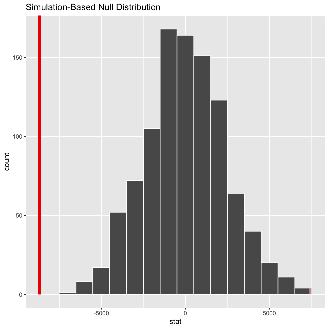

The infer package simulation supports the previous findings of the t.test and summary statistics. The observed mean falls very far away from the null distribution, so again we can reject the null hypothesis and conclude that there is strong evidence within the data set that gender has an impact in the salary of employees of Omega. There is a strong statistical difference between male salaries and female salaries, males earn on average 8696 units of currency more than their female counterparts.

Relationship Experience - Gender?

At the board meeting, someone raised the issue that there was indeed a substantial difference between male and female salaries, but that this was attributable to other reasons such as differences in experience. A questionnaire send out to the 50 executives in the sample reveals that the average experience of the men is approximately 21 years, whereas the women only have about 7 years experience on average (see table below).

# Summary Statistics of salary by gender
favstats (experience ~ gender, data=omega)

##   gender min    Q1 median   Q3 max  mean    sd  n missing
## 1 female   0  0.25    3.0 14.0  29  7.38  8.51 26       0
## 2   male   1 15.75   19.5 31.2  44 21.12 10.92 24       0

formula_ci <-mosaic::favstats (experience ~ gender, data=omega) 
formula_ci %>% 
mutate(t_critical = qt(0.975,n-1),
       SE = sd/sqrt(n),
       margin_of_error = t_critical*sd,
       low_endpoint  = mean - margin_of_error,
       high_endpoint = mean + margin_of_error)

##   gender min    Q1 median   Q3 max  mean    sd  n missing t_critical   SE
## 1 female   0  0.25    3.0 14.0  29  7.38  8.51 26       0       2.06 1.67
## 2   male   1 15.75   19.5 31.2  44 21.12 10.92 24       0       2.07 2.23
##   margin_of_error low_endpoint high_endpoint
## 1            17.5       -10.15          24.9
## 2            22.6        -1.46          43.7

Based on this evidence, can you conclude that there is a significant difference between the experience of the male and female executives? Perform similar analyses as in the previous section. Does your conclusion validate or endanger your conclusion about the difference in male and female salaries?

Answer: Based on the confidence interval analysis as above, because the t statistic is larger than the critical value 1.96 for 95% confidence interval, we should reject the null hypothesis and conclude that there is a significant difference between the experience of the male and female executives. Therefore, it could be the case that differences in experience between female and male contribute to difference in male and female salaries. The analysis here validates my conclusion about the difference in male and female salaries but we need to see the relationship between experience and salary.

Relationship Salary - Experience ?

Someone at the meeting argues that clearly, a more thorough analysis of the relationship between salary and experience is required before any conclusion can be drawn about whether there is any gender-based salary discrimination in the company.

Analyse the relationship between salary and experience. Draw a scatterplot to visually inspect the data

omega %>% 
  ggplot(aes(x = salary, y = experience, color=gender)) +
  geom_smooth(method = "lm", fill="grey90", size=4) + 
  geom_point(size=2) +
  theme_minimal() +
  labs(
    title = "Relationship between Salary and Experience, by Gender",
    subtitle = "Omega Salary Dataset",
    caption = "Omega Group plc- Pay Discrimination",
    x = "Salary", y = "Experience"
  )+ 
  coord_flip()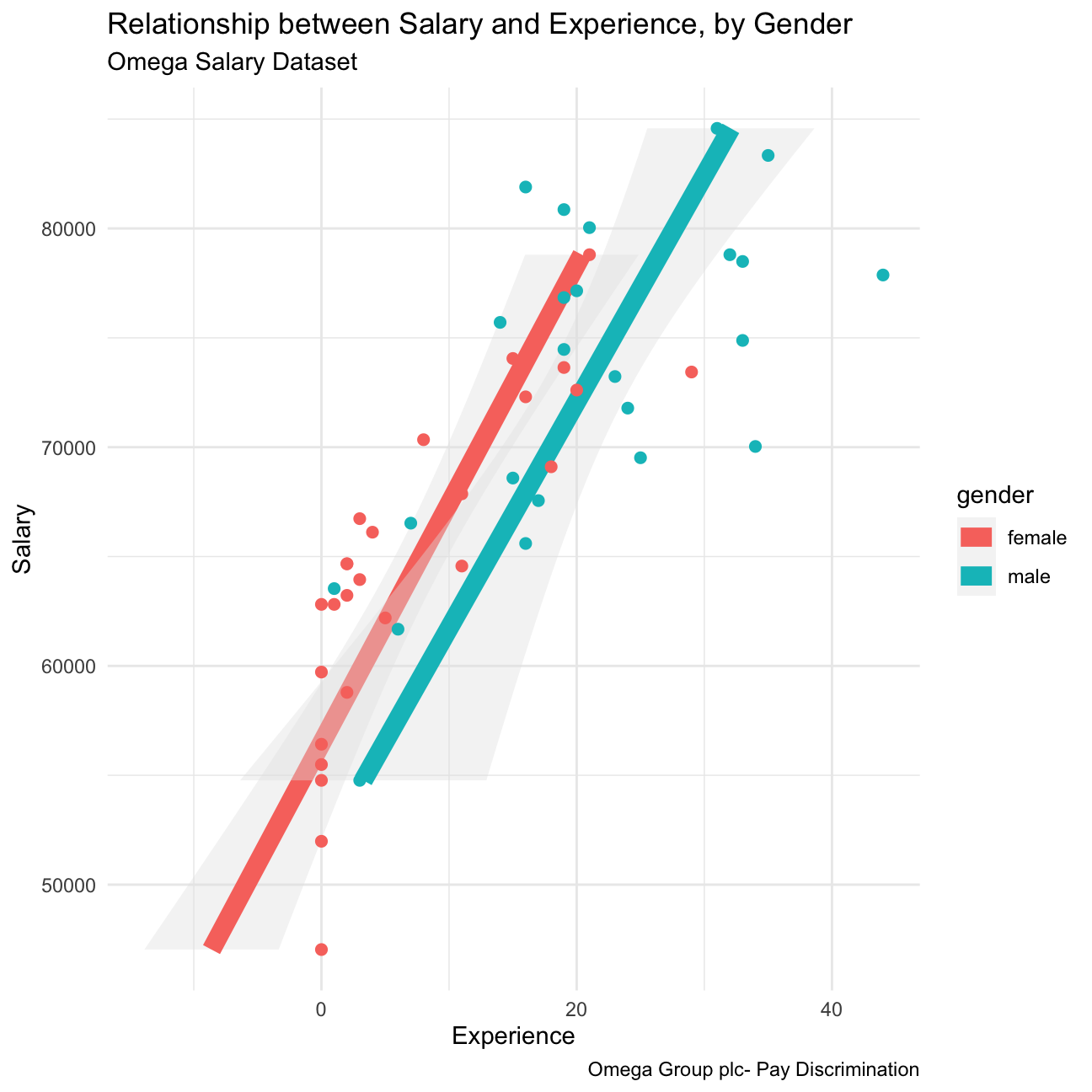

Check correlations between the data

You can use GGally:ggpairs() to create a scatterplot and correlation matrix. Essentially, we change the order our variables will appear in and have the dependent variable (Y), salary, as last in our list. We then pipe the dataframe to ggpairs() with aes arguments to colour by gender and make ths plots somewhat transparent (alpha = 0.3).

omega %>% 
  select(gender, experience, salary) %>% #order variables they will appear in ggpairs()
  ggpairs(aes(colour=gender, alpha = 0.3))+
  theme_bw()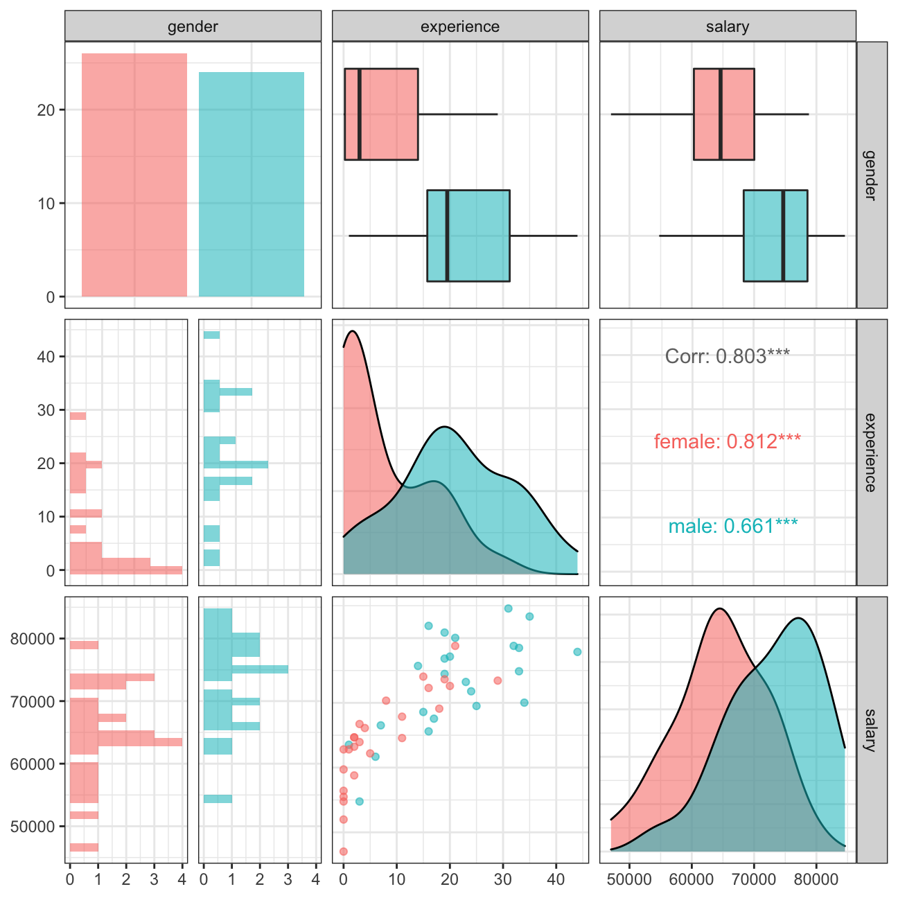

There is the positive correlation between salary and experience, and there seems to be a significant difference between the experience of the male and female executives on salary. To confirm this, we can also run the t-test and infer simulation to further support our findings.